Heatmap of Attack Directions

The code demonstrates how to extract the coordinates of a team’s attack directions and displays the points of arrival and intensity through a heatmap.

Setup

import of the needed libraries

Code

from datavolley import read_dv
import datavolley.pycourt as pycourt
import datavolley.pycourt as half_pycourt 
import matplotlib.pyplot as plt
import pandas as pd
import numpy as np
import seaborn as sns
import warnings
warnings.filterwarnings("ignore", "is_categorical_dtype")
warnings.filterwarnings("ignore", "use_inf_as_na")

Data reading

In this case, we will use the sample data that PyDataVolley is built upon and extract the actions using the get_plays() method.

Code

dvf = read_dv.DataVolley()
plays = dvf.get_plays()

Visualize the arrival of attacks

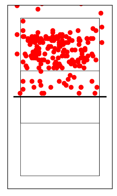
From the game actions we extract the information the x and y coordinates of the point of arrival of the attack. Our goal is to visualize the points where the ball arrives: where most of the play therefore takes place.

Code

attacks_data= plays[(plays['skill'] == 'Attack') & (plays.home_team==dvf.home_team)] 
coordinate_df = attacks_data[['end_coordinate_x','end_coordinate_y']]

def plot_coordinates(coordinates):
    pycourt.pycourt()
    # Plot the coordinates
    plt.scatter(coordinates['end_coordinate_x'], coordinates['end_coordinate_y'], color='red')
    plt.show(block=True)

plot_coordinates(coordinate_df)

Visualize the heatmap of attacks

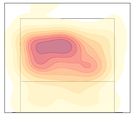
Using the same data we create the kernel density with seaborn and draw it on the field

Code

# heatmap of the end direction of attacks
fig, ax = plt.subplots()
pycourt.pycourt(ax)
sns.kdeplot(x=coordinate_df['end_coordinate_x'], y=coordinate_df['end_coordinate_y'], ax=ax, cmap="YlOrRd", fill=True, alpha=0.5)
plt.show()

Half a field

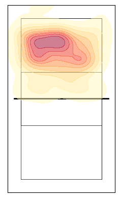
Among the functions available in pydatavolley is the ability to display half a court. Here we show how to use it

Code

# Creating the volleyball court
fig, ax = plt.subplots()
pycourt.half_pycourt(ax)
# Creating the heatmap
sns.kdeplot(x=coordinate_df['end_coordinate_x'], y=coordinate_df['end_coordinate_y'], ax=ax, cmap="YlOrRd", fill=True, alpha=0.5)
plt.show()

Code

df = plays[(plays['skill'] == 'Attack')]
total_attacks = df.groupby(['player_name', 'team']).size().reset_index(name='total')

Code

total_attacks

	player_name	team	total
0	Aiko Jones	University of Louisville	9
1	Alexa Hendricks	University of Louisville	8
2	Alli Papesh	University of Dayton	15
3	Amaya Tillman	University of Louisville	8
4	Amelia Moore	University of Dayton	9
5	Anna Stevenson	University of Louisville	11
6	Bridget Doherty	University of Dayton	3
7	Brooke Westbeld	University of Dayton	6
8	Claire Chaussee	University of Louisville	12
9	Emily Scott	University of Louisville	10
10	Jamie Peterson	University of Dayton	31
11	Jordan Albarran	University of Dayton	1
12	Mel McHenry	University of Louisville	23
13	Mikaylah Van Lanen	University of Dayton	2
14	Molly Asmus	University of Dayton	2
15	Olivia Dubay	University of Dayton	13
16	Player2 player2	University of Louisville	10
17	Rachael Fara	University of Dayton	10
18	Shannon Shields	University of Louisville	2
19	Sierra Pla	University of Dayton	5